Dynamics of Boolean Networks

In this tutorial, we study the dynamics of Boolean networks. Building on the construction and structural analysis from previous tutorials, we now focus on characterizing the long-term behavior of Boolean networks.

What you will learn

You will learn how to:

• simulate Boolean network dynamics under different updating schemes,

• compute and classify attractors,

• analyze basins of attraction,

• relate network structure to dynamical behavior.

Setup

import boolforge as bf
import numpy as np
import pandas as pd
import matplotlib.pyplot as plt

State space of a Boolean network

A Boolean network with \(N\) nodes defines a dynamical system on the discrete state space \(\{0,1\}^N\).

Each state is a binary vector

\[\mathbf{x} = (x_0, \ldots, x_{N-1}) \in \{0,1\}^N,\]

where \(x_i\) denotes the state of node \(i\).

We use a small Boolean network as a running example.

string = """
x = y
y = x OR z
z = y
"""

bn = bf.BooleanNetwork.from_string(string, separator="=")

print("Variables:", bn.variables)
print("N:", bn.N)
print("bn.I:", bn.I)
print("bn.F:")
for i, f in enumerate(bn.F):
    print(f"  F[{i}] = {f!r}")

Variables: ['x' 'y' 'z']
N: 3
bn.I: [array([1]), array([0, 2]), array([1])]
bn.F:
  F[0] = BooleanFunction(name='x', f=[0, 1])
  F[1] = BooleanFunction(name='y', f=[0, 1, 1, 1])
  F[2] = BooleanFunction(name='z', f=[0, 1])

All state vectors follow the variable order given by bn.variables. For small networks, we can enumerate all \(2^N\) states explicitly.

all_states = bf.get_left_side_of_truth_table(bn.N)
print(pd.DataFrame(all_states, columns=bn.variables).to_string())

   x  y  z
0  0  0  0
1  0  0  1
2  0  1  0
3  0  1  1
4  1  0  0
5  1  0  1
6  1  1  0
7  1  1  1

Dynamics of synchronous Boolean networks

Under synchronous updating, all nodes are updated simultaneously, defining a deterministic update map

\[\mathbf{x}(t+1) = F(\mathbf{x}(t)).\]

Exact computation

The update map \(F\) can be evaluated directly for any state vector. In BoolForge, this is implemented by the method update_network_synchronously. For convenience, Boolean networks are callable, so that bn(state) evaluates the update map and is equivalent to bn.update_network_synchronously(state).

for state in all_states:
    print(state, "-->", bn(state))

[0 0 0] --> [0 0 0]
[0 0 1] --> [0 1 0]
[0 1 0] --> [1 0 1]
[0 1 1] --> [1 1 1]
[1 0 0] --> [0 1 0]
[1 0 1] --> [0 1 0]
[1 1 0] --> [1 1 1]
[1 1 1] --> [1 1 1]

This output matches the synchronous truth table representation:

print(bn.to_truth_table().to_string())

   x(t)  y(t)  z(t)  x(t+1)  y(t+1)  z(t+1)
0     0     0     0       0       0       0
1     0     0     1       0       1       0
2     0     1     0       1       0       1
3     0     1     1       1       1       1
4     1     0     0       0       1       0
5     1     0     1       0       1       0
6     1     1     0       1       1       1
7     1     1     1       1       1       1

Each state has exactly one successor, so the dynamics consist of transient trajectories leading into attractors (steady states or cycles).

In this example, the network has:

• two steady states: \((0,0,0)\) and \((1,1,1)\),

• one cyclic attractor of length 2: \((0,1,0) \leftrightarrow (1,0,1)\).

Exhaustive attractor computation

BoolForge contains a dedicated method to identify all attractors of a network under synchronous update.

dict_dynamics = bn.get_attractors_synchronous_exact()

The returned dictionary contains:

• STG: the synchronous state transition graph,

• NumberOfAttractors,

• Attractors,

• AttractorID,

• BasinSizes.

For computational reasons, binary states in \(\{0,1\}^N\) are identified by their decimal representation. The state transition graph can be decoded as follows:

for state in range(2 ** bn.N):
    next_state = dict_dynamics["STG"][state]
    print(
        state,
        "=",
        bf.dec2bin(state, bn.N),
        "-->",
        next_state,
        "=",
        bf.dec2bin(next_state, bn.N),
    )

0 = [0, 0, 0] --> 0 = [0, 0, 0]
1 = [0, 0, 1] --> 2 = [0, 1, 0]
2 = [0, 1, 0] --> 5 = [1, 0, 1]
3 = [0, 1, 1] --> 7 = [1, 1, 1]
4 = [1, 0, 0] --> 2 = [0, 1, 0]
5 = [1, 0, 1] --> 2 = [0, 1, 0]
6 = [1, 1, 0] --> 7 = [1, 1, 1]
7 = [1, 1, 1] --> 7 = [1, 1, 1]

After repeated updates, the system settles into periodic behavior. That is, irrespective of the initial state, an attractor is reached. The list of all attractors (in decimal representation) can be displayed.

print(dict_dynamics['Attractors'])

[[0], [2, 5], [7]]

Attractors can be printed in binary representation:

for attractor in dict_dynamics["Attractors"]:
    print(f"Attractor of length {len(attractor)}:")
    for state in attractor:
        print(state, bf.dec2bin(state, bn.N))
    print()

Attractor of length 1:
0 [0, 0, 0]

Attractor of length 2:
2 [0, 1, 0]
5 [1, 0, 1]

Attractor of length 1:
7 [1, 1, 1]

The information which state transitions to which attractor is stored in a dictionary. Here, the indices correspond to the list of attractors in dict_dynamics['Attractors'].

for state_dec,attr_id in enumerate(dict_dynamics['AttractorID']):
    print(state_dec,'--> attractor',attr_id,
          'which is',dict_dynamics['Attractors'][attr_id])

0 --> attractor 0 which is [0]
1 --> attractor 1 which is [2, 5]
2 --> attractor 1 which is [2, 5]
3 --> attractor 2 which is [7]
4 --> attractor 1 which is [2, 5]
5 --> attractor 1 which is [2, 5]
6 --> attractor 2 which is [7]
7 --> attractor 2 which is [7]

Finally, the basin size of each attractor is determined by the number of states that eventually transition to an attractor. By definition, the sum of all basin sizes is always \(2^N\). To simplify the comparison of the basin size distribution for networks of different size, BoolForge normalizes the basin sizes by default.

print(dict_dynamics['BasinSizes'])

[0.125 0.5   0.375]

From the previous two outputs, we see that there is no state (other than 000) that eventually transitions to 000. Half the states transition to the 2-cycle, while 3 out of 8 states transition to the attractor 111.

Monte Carlo simulation

For larger networks, exhaustive enumeration is infeasible. Monte Carlo simulation approximates the attractor landscape.

dict_dynamics = bn.get_attractors_synchronous(n_simulations=1000)
print('Discovered attractors:',dict_dynamics['Attractors'])
print('Basin size approximation:',dict_dynamics['BasinSizesApproximation'])

Discovered attractors: [[7], [2, 5], [0]]
Basin size approximation: [0.383 0.498 0.119]

The simulation returns additional information:

• sampled initial states,

• the number of timeouts (trajectories not reaching an attractor before timeout).

for key in dict_dynamics:
    print(key)

Attractors
NumberOfAttractorsLowerBound
BasinSizesApproximation
AttractorID
InitialSamplePoints
STG
NumberOfTimeouts

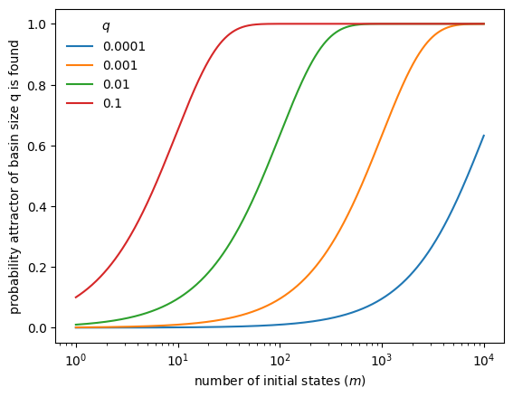
In the absence of timeouts: If an attractor has relative basin size \(q\), the probability that it is found from \(m\) random initializations is \(1 - (1-q)^m\).

qs = [0.0001, 0.001, 0.01, 0.1]
ms = np.logspace(0, 4, 1000)

fig, ax = plt.subplots()
for q in qs:
    ax.semilogx(ms, 1 - (1 - q) ** ms, label=str(q))

ax.legend(title=r"$q$", frameon=False)
ax.set_xlabel("number of initial states ($m$)")
ax.set_ylabel("probability attractor of basin size q is found")
plt.show()

Dynamics of asynchronous Boolean networks

Synchronous updating is computationally convenient but biologically unrealistic. Asynchronous updating assumes that only one node changes at a time.

Attractors under general asynchronous update

BoolForge can compute attractors under general asynchronous updating, where at each step only a single node updates according to its Boolean rule. Under synchronous updating, the dynamics are deterministic, while under asynchronous updating, the dynamics are generally stochastic. That implies that the notion of attractors needs to be adapted. In particular, synchronous limit cycles typically disappear under asynchronous updating, while steady states remain unchanged. Instead, under asynchronous updating, the long-term behavior is characterized by the terminal strongly connected components (SCCs) of the asynchronous state transition graph.

terminal_sccs = bn.get_terminal_sccs_asynchronous_exact()
print('Terminal strongly connected components:', terminal_sccs)

Terminal strongly connected components: [[0], [7]]

The result reveals the same two steady states as in the synchronous case. However, the limit cycle observed under synchronous updating disappears under asynchronous dynamics.

In addition, BoolForge can return the full asynchronous state transition graph.

STG_async = bn.get_asynchronous_transition_matrix()
print(STG_async)

<Compressed Sparse Row sparse matrix of dtype 'float32'
        with 14 stored elements and shape (8, 8)>
  Coords        Values
  (0, 0)        1.0
  (1, 0)        0.5
  (1, 3)        0.5
  (2, 0)        0.3333333432674408
  (2, 3)        0.3333333432674408
  (2, 6)        0.3333333432674408
  (3, 7)        1.0
  (4, 0)        0.5
  (4, 6)        0.5
  (5, 1)        0.3333333432674408
  (5, 4)        0.3333333432674408
  (5, 7)        0.3333333432674408
  (6, 7)        1.0
  (7, 7)        1.0

The state transition graph, a sparse transition matrix of a Markov chain, describes all possible state transitions, together with their probabilities.

From this matrix, BoolForge can compute the absorption probabilities, i.e., the probability that a trajectory starting from a given state eventually reaches a specific terminal SCC.

print(np.round(bn.get_absorption_probabilities_exact(),4))

[[1.     0.    ]
 [0.5    0.5   ]
 [0.3333 0.6667]
 [0.     1.    ]
 [0.5    0.5   ]
 [0.3333 0.6667]
 [0.     1.    ]
 [0.     1.    ]]

This shows that the state 001 (1 in decimal representation) reaches both steady states with equal probability. On the other hand, the states 011 (decimal = 3) and 110 (decimal = 6) always eventually settle in the steady state 111, the second attractor in terminal_sccs.

From the absorption probabilities, the size of each basin of attraction can also be readily computed as the column-wise sum of these probabilities. This metric, together with many other dynamical properties, is returned by the method get_terminal_sccs_and_robustness_asynchronous_exact, which we investigate in more detail in the next tutorial.

dict_dynamics = bn.get_terminal_sccs_and_robustness_asynchronous_exact()
print('Basin sizes:',dict_dynamics['BasinSizes'])

Basin sizes: [0.33333334 0.6666666 ]

Monte Carlo approximation

As in the synchronous case, BoolForge also contains a Monte Carlo routine for sampling asynchronous dynamics. However, this routine is currently limited to identifying steady states and approximating their basin sizes. It does not identify terminal SCCs. For this task, specialized tools such as pystablemotifs are recommended [@rozum2022pystablemotifs].

BoolForge’s simulation framework provides:

• a lower bound on the number of steady states,

• approximate basin size distributions,

dict_dynamics = bn.get_steady_states_asynchronous(n_simulations=500)
print('Discovered steady states:', dict_dynamics['SteadyStates'])
print('Number of steady states (lower bound):',dict_dynamics['NumberOfSteadyStatesLowerBound'])
print('Basin size approximation:',dict_dynamics['BasinSizesApproximation'])

Discovered steady states: [7, 0]
Number of steady states (lower bound): 2
Basin size approximation: [0.68 0.32]

Sampling from a fixed initial condition

In biological Boolean network models, a specific state \(\mathbf x \in \{0,1\}^N\) is frequently considered the initial state, e.g., corresponding to the G0 phase of the cell cylce. To enable exploration of the stochastic trajectories from a specific state, BoolForge contains the following method.

dict_dynamics = bn.get_steady_states_asynchronous_given_one_initial_condition(
    initial_condition=[0, 0, 1], n_simulations=500
)
print('Discovered steady states:', dict_dynamics['SteadyStates'])
print('Number of steady states (lower bound):',dict_dynamics['NumberOfSteadyStatesLowerBound'])
print('Basin size approximation:',dict_dynamics['BasinSizesApproximation'])

Discovered steady states: [0, 7]
Number of steady states (lower bound): 2
Basin size approximation: [0.526 0.474]

Note the equivalent analysis under synchronous update is trivial because the dynamics are deterministic and the long-term behavior when starting in a specific initial condition can be found by

dict_dynamics = bn.get_attractors_synchronous(n_simulations=1,
                                              initial_sample_points=[[0,0,1]],
                                              initial_sample_points_are_vectors=True)
for key, value in dict_dynamics.items():
    print(f"{key}: {value}")

Attractors: [[2, 5]]
NumberOfAttractorsLowerBound: 1
BasinSizesApproximation: [1.]
AttractorID: {2: 0, 5: 0}
InitialSamplePoints: [[0, 0, 1]]
STG: {1: 2}
NumberOfTimeouts: 0

Summary

In this tutorial you learned how to:

• simulate Boolean network dynamics,

• compute synchronous attractors exactly and approximately,

• analyze basin sizes,

• compute asynchronous attractors (terminal SCCs) and absorption probabilities exactly,

• identify, by simulation, some (but possible not all) steady states for large asynchronously updated Boolean networks.

This concludes the function- and network-level analysis. Subsequent tutorials focus on analyzing stability to perturbations, control analysis, and ensemble experiments.